I’ve been working on a Bayesian implementation of Joe Pickrell and Jonathan Pritchard’s admixture model (implemented as TreeMix). Their model extends Cavalli-Sforza and Edwards’ seminal work on phylogenetic analysis, which assumed that modern populations allele frequencies evolved according to a Brownian motion model and covary according to an underlying bifurcating tree. By permitting admixture edges, the Pickrell-Pritchard model can capture signals of gene flow in cases where a bifurcating tree describes covariance in the populations’ allele frequencies poorly (which is anything but a rare occurrence in, say, humans). These admixture edges transform our beautiful (though biologically unrealistic) bifurcating tree into a less wieldy tree-like graph. While phylogenetics have used consensus trees to describe topological uncertainty, I couldn’t find a good way to summarize uncertainty for this sort of tree-like directed acyclic graph (DAG).
One approach I’m exploring is to plot the majority rule consensus tree for the underlying bifurcating divergence tree. Then conditioning on that tree, plot the admixture edges with posterior probability greater than, say, 0.5 given that the source and destination branches exist. This gives you a conditioned majority rule consensus DAG of sorts.
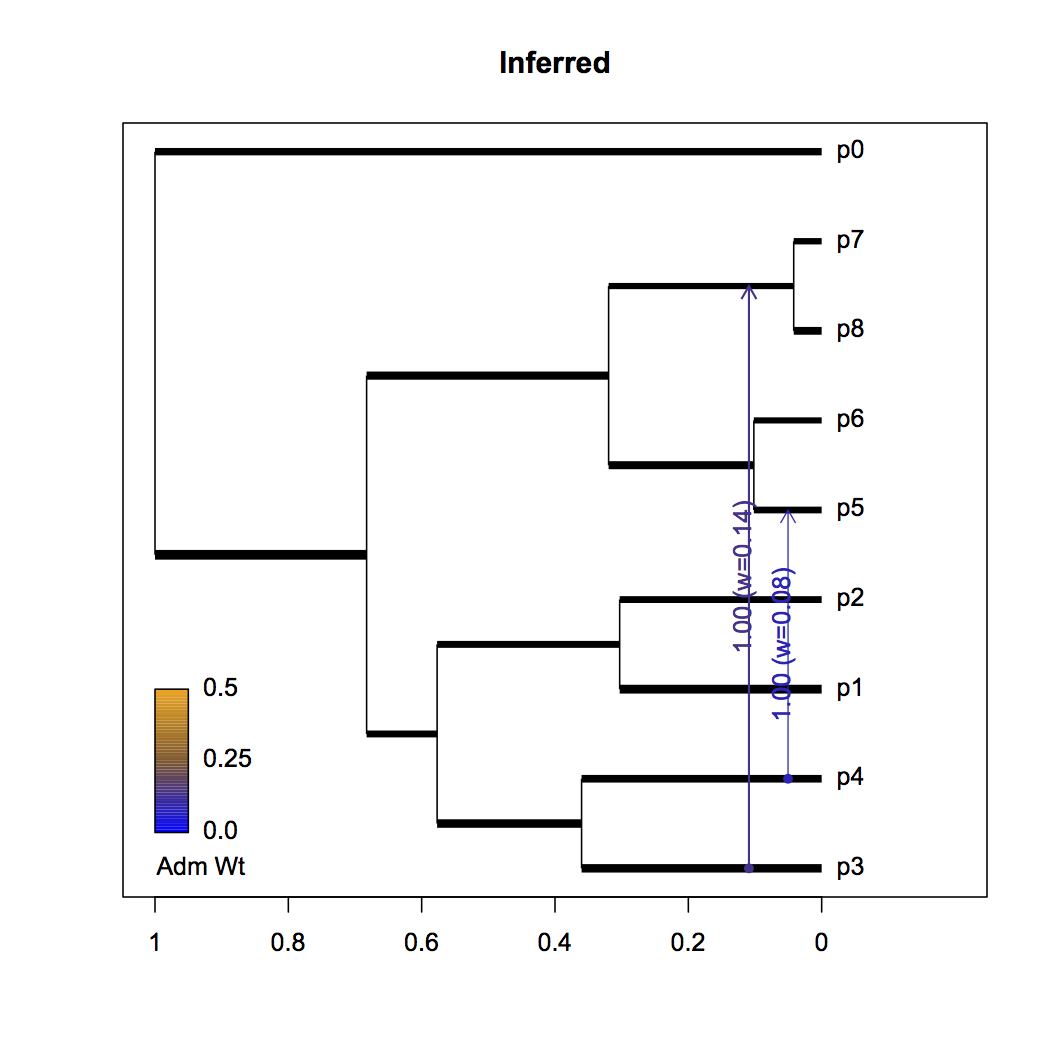
Now, I’ve been interested in how well this method works for only a single diploid sample per population, so data was simulated for 20 populations with two samples per population and 100000 SNPs per sample. You can see the resulting conditioned majority rule consensus DAG below, generated by some R scripts that parse RevBayes’ MCMC output.
The tree height is one, but scaled by a parameter that captures information about the mean population size, time to the most recent common ancestor, and generation time (not shown). Branch lengths are proportional to time and widths are informative of population size relative to the population size mean (log scale). All divergence events were supported with posterior probability 1.0, so those values are not shown. Although time and population size aren’t identifiable, they are useful to separate since I model admixture events to occur instantaneously in time. Admixture edges report their posterior probability and mean posterior admixture weight.
What’s important to note is that the analysis records the admixture edges p4->p5 and p3->(p7,p8) as having high posterior probability. There’s some uncertainty in the exact placement of edge p3->(p7,p8). The order of admixture events is reversed, partly owing to the non-identifiability of age from population size. Finally, since population size and time aren’t identifiable and are inversely related, we see the model redistributes these parameter values fairly evenly (notably, the sister lineage to p0 is lengthened, possibly due to the birth-death prior on divergence times).
True graph:

Inferred graph: